## Latest release from CRAN
 install.packages("brms")

## Or the latest development version from GitHub
 devtools::install_github("paul-buerkner/brms")
brms in application
brms - a package that can help you throughout your Bayesian workflow!
brms (short for Bayesian Regression Models using ‘Stan’) is a package that allows for user friendly specification of Bayesian models. The package was developed by Paul-Christian Bürkner. If you are mostly familiar with linear regression of the frequentist sort, you are in luck: the formula syntax in brms is very similar to that in lme4! The brms README file links to several resources including extensive package documentation, vignettes, and forum discussions
If you are new to Bayesian stats or are in need of a little brush up, check out this Bayesian Primer by Van de Schoot et al. (2021).
Install brms
You will first need to download brms.
brms & the Bayesian workflow
1. Pick an initial model
brm is the modelling function where you can specify anything that may be relevant to your model (e.g., the response distribution, priors, group-level factors, number of chains, iterations, etc.).
Some of the core arguments you will need to specify are:
formula: this is where you specify your response and predictor variables of interest (e.g., y ~ x). This is also where you will specify your random effects (e.g., y ~ x1 + (1|x2)data: specify your dataframefamily: brms can handle a wide range of response distributions linear, count data, survival, response times, ordinal, zero-inflated, self-defined mixture models and much much more! This is also where you specify yourlinkargument
Other arguments you might want to specify:
prior: specify the prior distributions you would like for your population-level and group-level variables. You are also not restricted to just normal distributions and specify different types including uniform, Cauchy, Gamma, etc. If you do not specify your priors, the model assumes a prior with a student_t distribution.warmup: number of burn in iterations to help model find stable sampling space (default is iter/2)iter:number of total iterations per chain (default is 2000)chains: number of markov chains you would like to run (default is 4)cores: number of cores to use when chains are running (default is 1), but you may want to specify more if your computer has capability. You can check how many cores you have by using parallel::detectCores()control:adjust the sampling behavior of the model. I’ve mostly used this to help lower the number of divergent transitions (e.g., control = list(adapt_delta(x=.9)))file:you can tell the model where to save its results (e.g., file = paste0(model,“/m_results”)
Another modelling function is brm_multiple for when you have multiple datasets that you would like to run your model over. Specifically, this is helpful if you missing data and your dataset would benefit from multiple imputation. brms interfaces nicely with the mice package which allows you to pass multiple imputed datasets into your model which then combines the posteriors draws into one model result. You can then run the rest of the brms post-processing methods as you typically would.
2. Fit the model
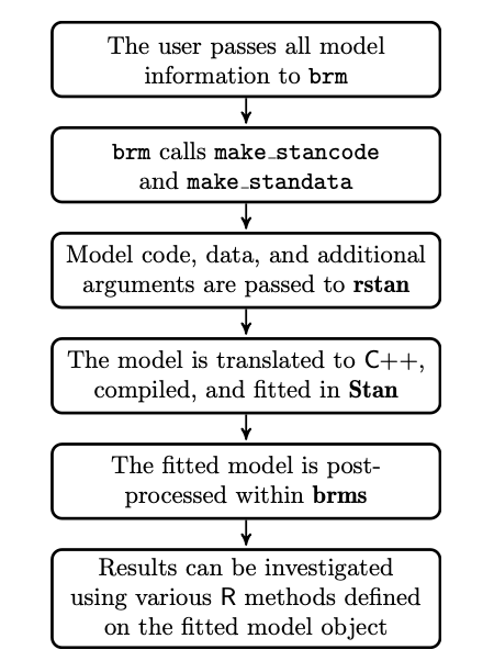
Figure 1. brms model fitting procedure (Burkner, 2017)
3. Validate computation
This part of the workflow stresses the use of simulated data to make sure the model takes a reasonable length of time to run & passes convergence diagnostics.
Check out your model results: the summary function will spit out key model information like the family, formula, data and number of observations used in the model, number of samples, WAIC score, population-level effects and group-level effects (if you have any) with their respective estimates, error, 95% confidence interval, effective sample size, and Rhat score.
Effective sample size and Rhat score are two default metrics of convergence. If your effective sample size is much lower than your number of iterations there could be efficiency issues in your chains. Secondly, if your Rhat score is > 1, then this indicates some convergence issues and therefore may not have reliable results.
4. Address computational issues
In general, it is helpful to start with a simple version of the model to diagnose exactly where you are running into issues. Within your argument specification in the brm function, you can play around with the following:
If your model is taking a long time to run, try a smaller simulated dataset or a subset of your data, lower the number of
iterfrom the default (which is 2000), or add in more informative priors than you had previously by adjusting thepriorargument.If your model is having convergence issues, you can try adjusting the
controlfunction to be greater than the default, which is .8, up to 1.
5. Evaluate and use model OR modify the model
There are a couple of functions from the bayesplot package that interface with brms to evaluate your model. Most commonly, I will use the following functions to assess my model:
Posterior predictive checking is one way to see how your model results compare with your observed data. You can run a posterior predictive check with the
pp_checkand specify several different types of checks. The most common ones I use are: “dens_overlay” and “intervals_grouped” if I am running a mixed model.Trace plot for your model using
mcmc_plotto see if there was adequate chain mixing.
Another good test is leave-one-out cross-validation (LOOCV). LOOCV essentially checks the predictive ability of your model when part of the data is left out. This is helpful for understanding the influence of certain observations on your model fit. You can test on your model with loo.
6. Compare models
Keep all your model iterations. You can think of the Bayesian workflow as a process, where anything you do in this workflow is information about your data analysis.
brms aims to make it straightforward to adjust aspects of your model (e.g., model equation, priors, number of iterations) so that you can make comparisons between them. Once you have some models that you would like to compare, you can run loo_compare to see had the best predictive ability or run your other evaluation checks to compare fit.