Example: penguins

Let’s look at an example. We will load a dataset and make a regression model.

Penguin data

Begin by installing the palmerpenguins package from Allison Horst’s Github. Then load the package and import the data.

# install the palmerpenguins package
remotes::install_github("allisonhorst/palmerpenguins")
library( "palmerpenguins" )
data( penguins )

Estimate a linear model

Here’s a common task: estimate a linear regression model for some data. The result is an object (one that uses the S3 system)

# make a linear regression model:
penguin_lm = lm( body_mass_g ~ species + sex, data=penguins )

# check the lm object:
is.object( penguin_lm )

[1] TRUE

attr( penguin_lm, "class" )

[1] "lm"

class( penguin_lm )

[1] "lm"

The plot() function does more than one thing

What happens when you call the plot() function depends on what kind of object you are plotting. This had to be built into R! Functions only do what they are told, so how can plot() do different things?!

# plot the data and the model
plot( penguins )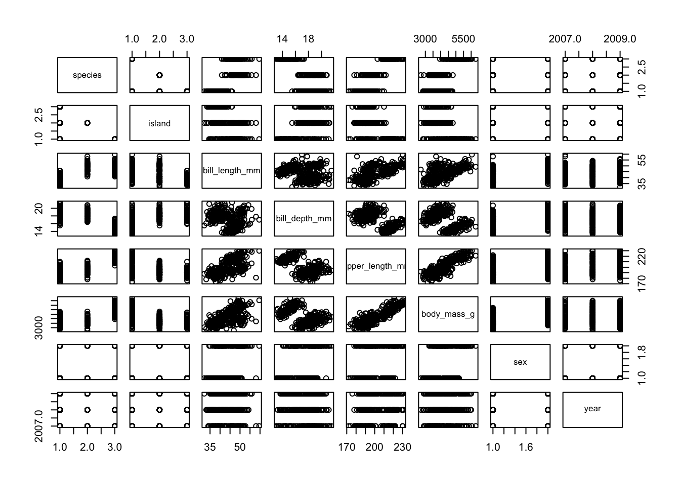

layout( matrix(1:4, 2, 2))
plot( penguin_lm )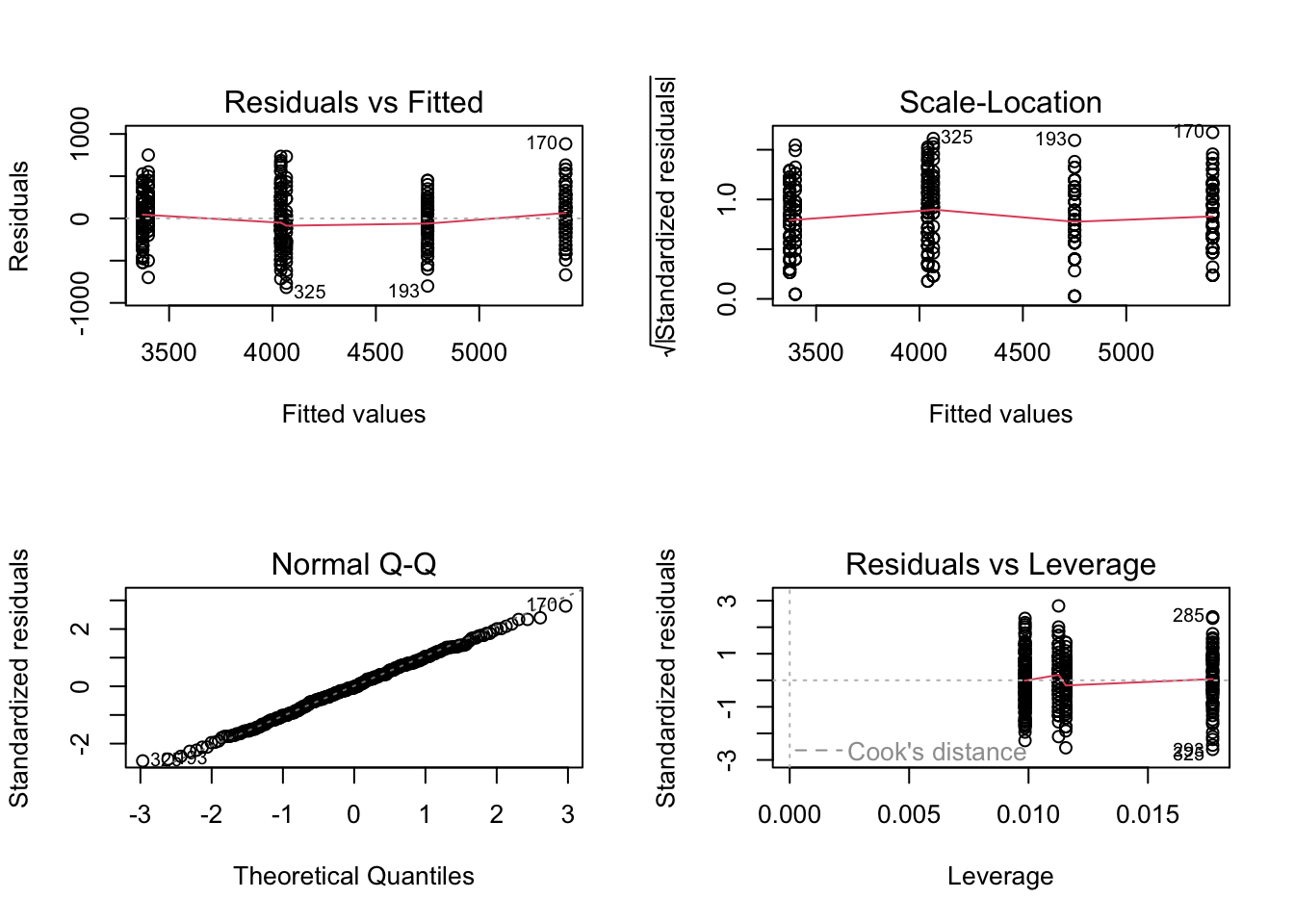

The summary() function does more than one thing

Similarly, the summary() function can do different things depending on what object it works on. On a data.frame, summary() will summarize each column. Called on a fitted linear model, summary() will tell you about the coefficients, their significange levels, and calculate the model’s R-squared.

# summarize the data and the model
summary( penguins )

      species          island    bill_length_mm  bill_depth_mm  
 Adelie   :152   Biscoe   :168   Min.   :32.10   Min.   :13.10  
 Chinstrap: 68   Dream    :124   1st Qu.:39.23   1st Qu.:15.60  
 Gentoo   :124   Torgersen: 52   Median :44.45   Median :17.30  
                                 Mean   :43.92   Mean   :17.15  
                                 3rd Qu.:48.50   3rd Qu.:18.70  
                                 Max.   :59.60   Max.   :21.50  
                                 NA's   :2       NA's   :2      
 flipper_length_mm  body_mass_g       sex           year     
 Min.   :172.0     Min.   :2700   female:165   Min.   :2007  
 1st Qu.:190.0     1st Qu.:3550   male  :168   1st Qu.:2007  
 Median :197.0     Median :4050   NA's  : 11   Median :2008  
 Mean   :200.9     Mean   :4202                Mean   :2008  
 3rd Qu.:213.0     3rd Qu.:4750                3rd Qu.:2009  
 Max.   :231.0     Max.   :6300                Max.   :2009  
 NA's   :2         NA's   :2                                 

summary( penguin_lm )

Call:
lm(formula = body_mass_g ~ species + sex, data = penguins)

Residuals:
    Min      1Q  Median      3Q     Max 
-816.87 -217.80  -16.87  227.61  882.20 

Coefficients:
                 Estimate Std. Error t value Pr(>|t|)    
(Intercept)       3372.39      31.43 107.308   <2e-16 ***
speciesChinstrap    26.92      46.48   0.579    0.563    
speciesGentoo     1377.86      39.10  35.236   <2e-16 ***
sexmale            667.56      34.70  19.236   <2e-16 ***
---
Signif. codes:  0 '***' 0.001 '**' 0.01 '*' 0.05 '.' 0.1 ' ' 1

Residual standard error: 316.6 on 329 degrees of freedom
  (11 observations deleted due to missingness)
Multiple R-squared:  0.8468,    Adjusted R-squared:  0.8454 
F-statistic: 606.1 on 3 and 329 DF,  p-value: < 2.2e-16

An lm object encapsulates many pieces

The linear model object penguin_lm contains a lot of pieces. You can see the names of the pieces by using the names() function.

# access some pieces that are encapsulated in the model:
names( penguin_lm )

 [1] "coefficients"  "residuals"     "effects"       "rank"         
 [5] "fitted.values" "assign"        "qr"            "df.residual"  
 [9] "na.action"     "contrasts"     "xlevels"       "call"         
[13] "terms"         "model"        

penguin_lm$coefficients

     (Intercept) speciesChinstrap    speciesGentoo          sexmale 
      3372.38681         26.92385       1377.85803        667.55515 

penguin_lm$call

lm(formula = body_mass_g ~ species + sex, data = penguins)